CytoProfile is an R package designed for end-to-end analysis and visualization of cytokine profiling data from immunological and clinical studies. It provides a structured workflow covering:
- Quality control and distributional assessment
- Exploratory visualization (boxplots, violin plots, error bar plots)
- Univariate statistical testing (t-test / Wilcoxon, ANOVA / Kruskal-Wallis)
- Multivariate methods (PCA, sPLS-DA, MINT sPLS-DA)
- Statistical visualizations (volcano plots, heatmaps, dual-flashlight plots)
- Machine learning classification (Random Forest, XGBoost)
This vignette provides a guided, step-by-step tutorial for each function, including input data requirements, key parameters, and guidance on interpreting outputs.
Installation and Dependencies
Required Bioconductor package
CytoProfile depends on mixOmics, which must be installed from Bioconductor before installing CytoProfile:
if (!requireNamespace("BiocManager", quietly = TRUE)) {
  install.packages("BiocManager")
}
BiocManager::install("mixOmics")
Installing CytoProfile
# From CRAN (stable release)
install.packages("CytoProfile")

# From GitHub (development version)
# install.packages("devtools")
devtools::install_github("saraswatsh/CytoProfile", ref = "devel")
Package loading
CytoProfile imports all necessary packages internally, you do
not need to call library() for its
dependencies (e.g., ggplot2, dplyr,
mixOmics). The only exception in this vignette is
dplyr, which is used explicitly for data subsetting in the
examples below and is not re-exported by CytoProfile.
library(CytoProfile)
library(dplyr)   # used only for filter() in the examples below
1. Data Loading and Format Requirements
Input data format
All CytoProfile functions expect a data frame (or coercible matrix) where:
- Cytokine columns are numeric (concentrations or transformed values).
- Grouping columns (e.g., disease group, treatment) are character or factor.
- There are no strict naming requirements, but column
names must be unique. The functions internally call
make.names()to sanitize names with special characters (e.g.,CCL-20/MIP-3AbecomesCCL.20.MIP.3A). - Missing values (
NA) are handled internally by most functions, but rows with all-missing cytokine values should be removed prior to analysis.
CytoProfile ships with five example datasets
(ExampleData1 through ExampleData5).
Throughout this vignette we use ExampleData1, which
contains 297 observations of 25 cytokines along with Group,
Treatment, and Time columns.
data("ExampleData1")
data_df <- ExampleData1

# Inspect structure
dim(data_df)
#> [1] 297  28
names(data_df)[1:6]
#> [1] "Group"     "Treatment" "Time"      "IL-17F"    "GM-CSF"    "IFN-G"
head(data_df[, 1:5])
#>   Group Treatment Time IL-17F GM-CSF
#> 1   T2D  CD3/CD28   20   3.31   7.16
#> 2   T2D  CD3/CD28   20   0.38   0.87
#> 3   T2D  CD3/CD28   20   1.25   2.47
#> 4   T2D  CD3/CD28   20   2.24   3.52
#> 5   T2D  CD3/CD28   20   0.25   1.58
#> 6   T2D  CD3/CD28   20   0.96   1.87
table(data_df$Group)
#>
#>     ND PreT2D    T2D
#>     99     99     99
table(data_df$Treatment)
#>
#>     CD3/CD28          LPS Unstimulated
#>           99           99           99
Recommended sample size: Functions perform best with at least 10 samples per group. Machine learning functions (Random Forest, XGBoost) require larger sample sizes ( 20 per group) to produce reliable cross-validated performance estimates.
2. Exploratory Data Analysis
2.1 Boxplots - cyt_bp()
Purpose: Generate boxplots for each numeric variable, optionally grouped by one or more categorical variables.
Key data requirements: - At least one numeric column
is required. - If group_by is specified, those columns must
be character or factor.
Key parameters:
| Parameter | Description | Default |
|---|---|---|
data |
Data frame or matrix | - |
group_by |
Column name(s) for grouping | NULL |
scale |
Transformation: "none", "log2",
"log10", "zscore", "custom"
|
"none" |
bin_size |
Max plots per page (ungrouped only) | 25 |
y_lim |
y-axis limits, e.g. c(0, 20)
|
NULL |
output_file |
File path to save (e.g. "plots.pdf"). NULL
displays interactively. |
NULL |
When to use which scale: -
"log2" or "log10": when cytokine
concentrations span several orders of magnitude or show strong
right-skew (common for raw immunoassay data). - "zscore":
when comparing distributions on a standardized scale across cytokines
with very different concentration ranges. - "none": when
data are already transformed.
Interpreting the output: - Each boxplot shows the median (horizontal line), interquartile range (box), 1.5x IQR whiskers, and individual data points (jittered). - Overlapping distributions between groups suggest no strong group effect for that cytokine. - Outliers far beyond the whiskers warrant attention - consider whether they represent biological extremes or measurement artefacts.
# Ungrouped boxplots with log2 transformation
# All numeric columns are plotted; up to bin_size = 25 per page
cyt_bp(data_df[, -c(1:3)], output_file = NULL, scale = "log2")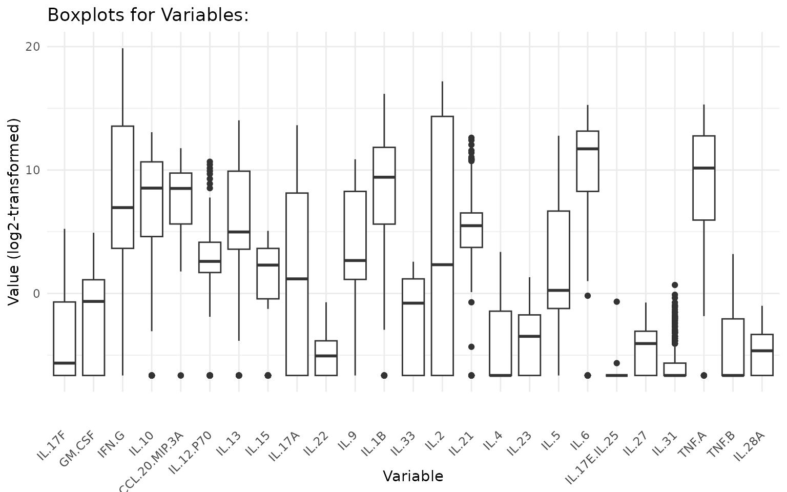
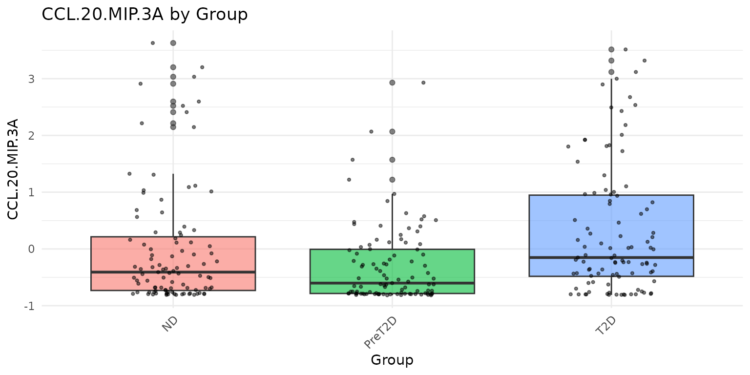
# Grouped boxplots: one plot per cytokine, colored by Group
# Only passing Group and two cytokines for a concise display
cyt_bp(
  data_df[, c("Group", "IL-10", "CCL-20/MIP-3A")],
  group_by = "Group",
  scale = "zscore"
)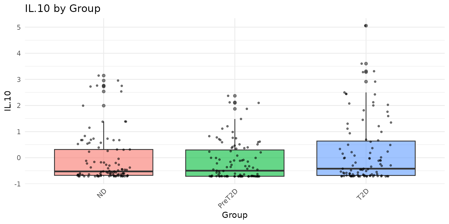
Note:
cyt_bp()invisibly returns a named list ofggplotobjects, so you can retrieve and further modify any individual plot:plots <- cyt_bp(...); plots[["IL-10"]] + ggplot2::ggtitle("Custom title").
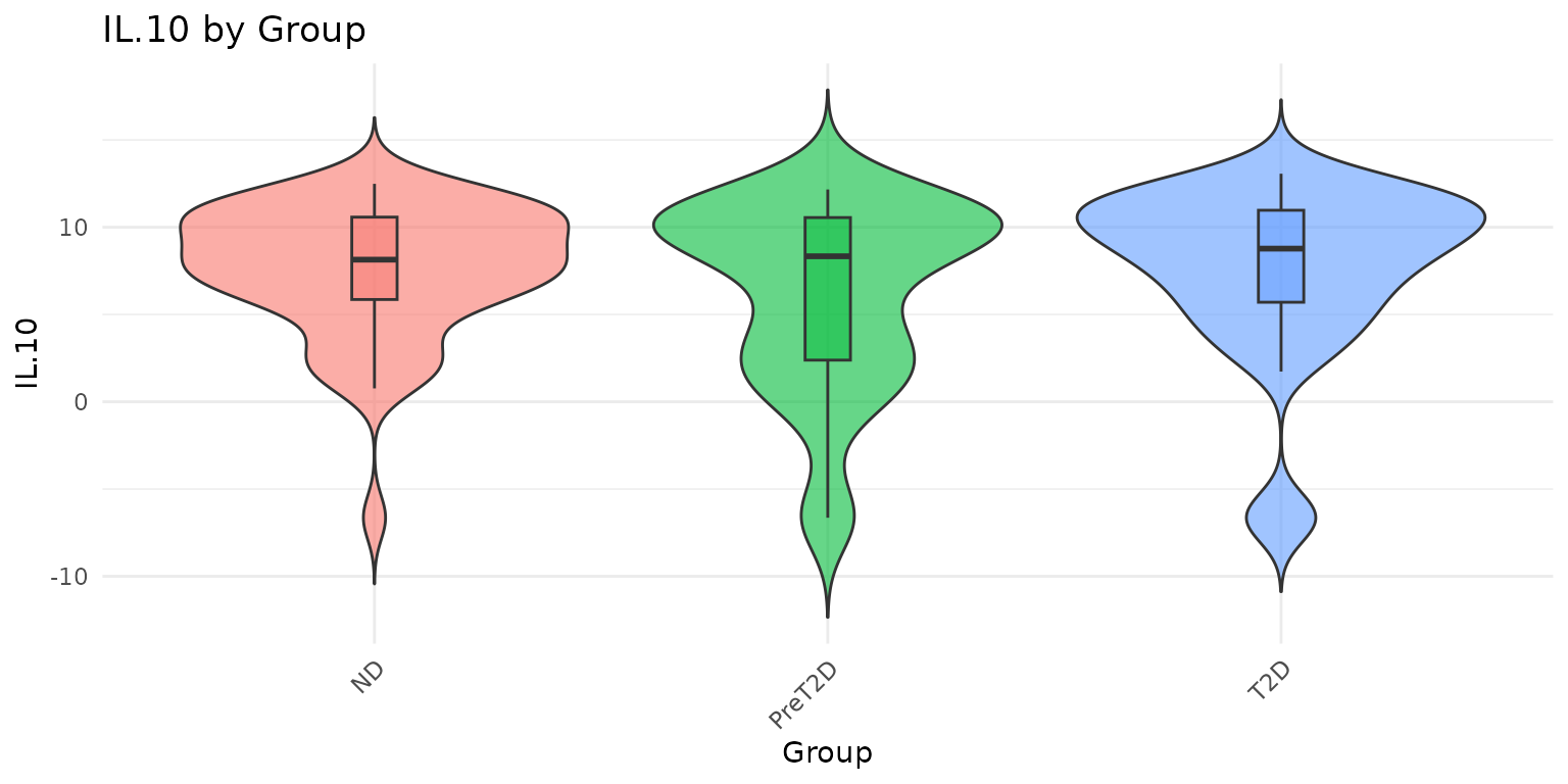
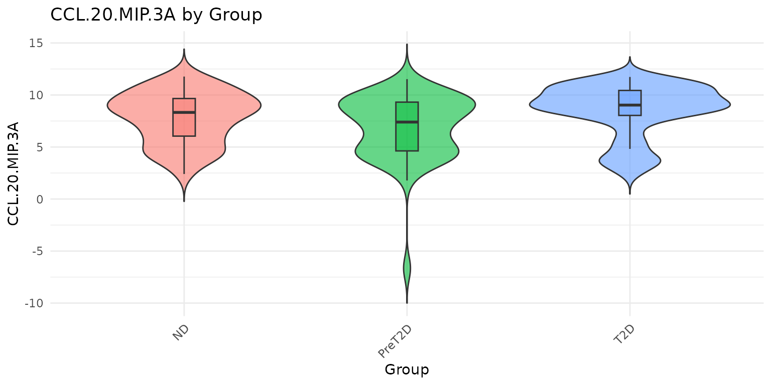
2.2 Violin Plots - cyt_violin()
Purpose: Similar to cyt_bp() but shows
the full data distribution shape using kernel density estimation, making
it especially informative for bimodal or asymmetric cytokine
distributions.
Key parameters (same as cyt_bp(),
plus):
| Parameter | Description | Default |
|---|---|---|
boxplot_overlay |
Draw a narrow boxplot inside each violin to show median and IQR | FALSE |
Interpreting the output: - A wide violin belly
indicates many observations at that value. - Bimodal violins (two wide
regions) suggest subpopulations within a group - worth investigating
with further stratification. - Setting
boxplot_overlay = TRUE combines density estimation with
quartile summaries in one panel.
# Ungrouped violin plots with z-score scaling
cyt_violin(data_df[, -c(1:3)], output_file = NULL, scale = "zscore")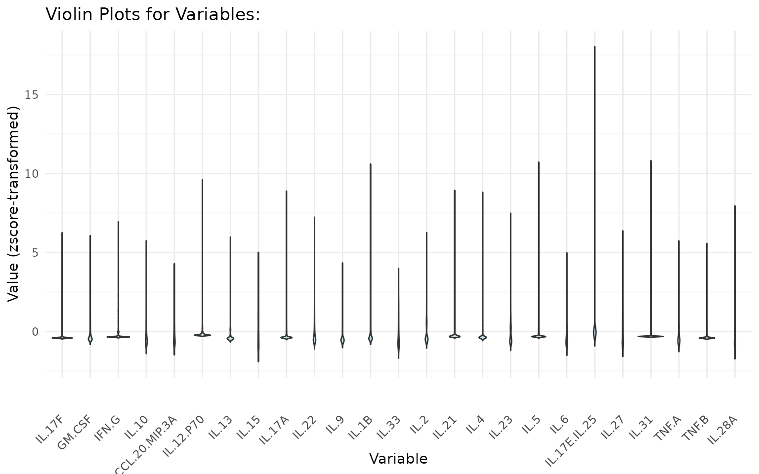
# Grouped violin plots with boxplot overlay and log2 scaling
cyt_violin(
  data_df[, c("Group", "IL-10", "CCL-20/MIP-3A")],
  group_by = "Group",
  boxplot_overlay = TRUE,
  scale = "log2"
)
2.3 Skewness and Kurtosis - cyt_skku()
Purpose: Assess whether cytokine distributions are symmetric (skewness 0) and whether they have tails heavier than a normal distribution (kurtosis > 0). This is important for deciding whether a log or other transformation is appropriate before statistical testing.
Key data requirements: - Numeric measurement columns
only (exclude grouping columns via group_cols). - All
values should be positive if log2 transformation will be applied
downstream, since cyt_skku() uses log2 internally for
comparison.
Key parameters:
| Parameter | Description | Default |
|---|---|---|
group_cols |
Character vector of grouping column names | NULL |
print_res_raw |
Return summary stats for raw data | FALSE |
print_res_log |
Return summary stats for log2-transformed data | FALSE |
output_file |
File path to save plots | NULL |
Interpreting the output: - Two histograms are produced: one for skewness, one for kurtosis, comparing raw data (red) and log2-transformed data (blue). - Skewness: Values far from 0 indicate asymmetry. Positive skewness (right tail) is common in raw cytokine data. After log2 transformation, distributions closer to 0 indicate better symmetry. - Kurtosis: Positive excess kurtosis indicates heavier-than-normal tails (more outliers expected). After log2 transformation, kurtosis values closer to 0 suggest the transformation improved normality. - If log2 transformation substantially reduces both skewness and kurtosis compared to raw values, it is recommended as a pre-processing step.
# Overall distributional assessment (no grouping)
cyt_skku(data_df[, -c(1:3)], output_file = NULL, group_cols = NULL)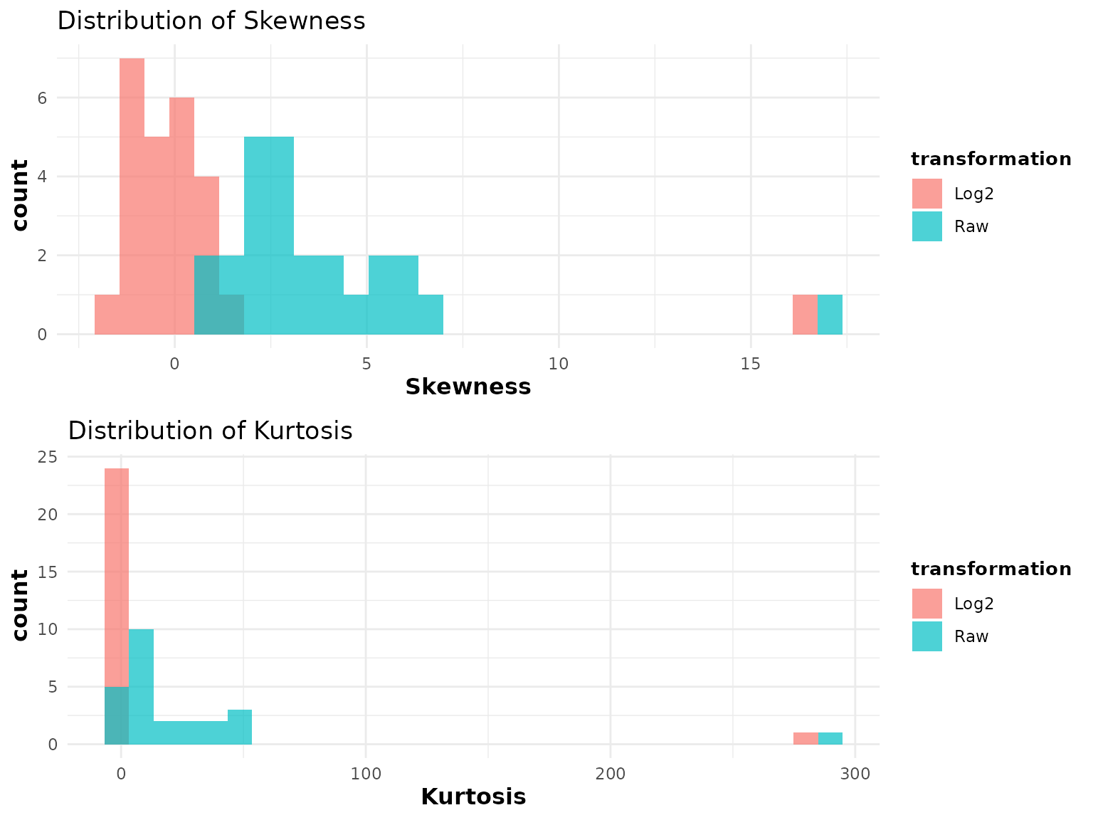
# Grouped assessment by "Group"
cyt_skku(data_df[, -c(2:3)], output_file = NULL, group_cols = c("Group"))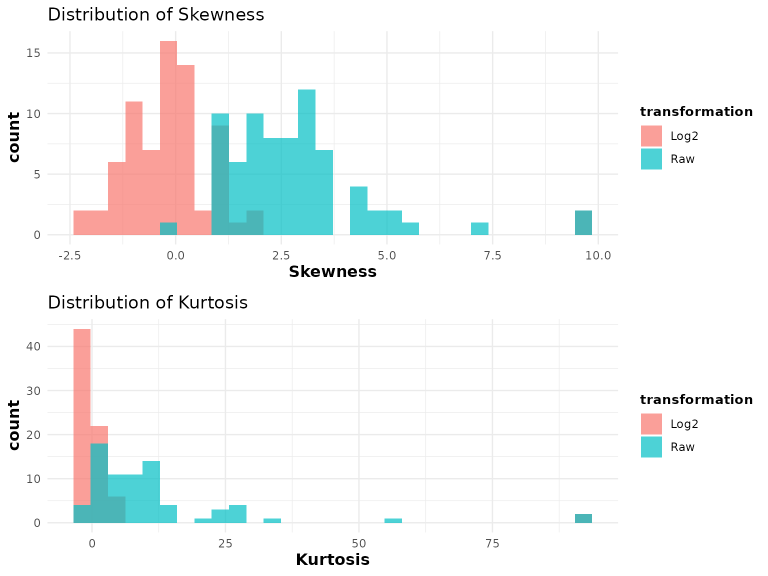
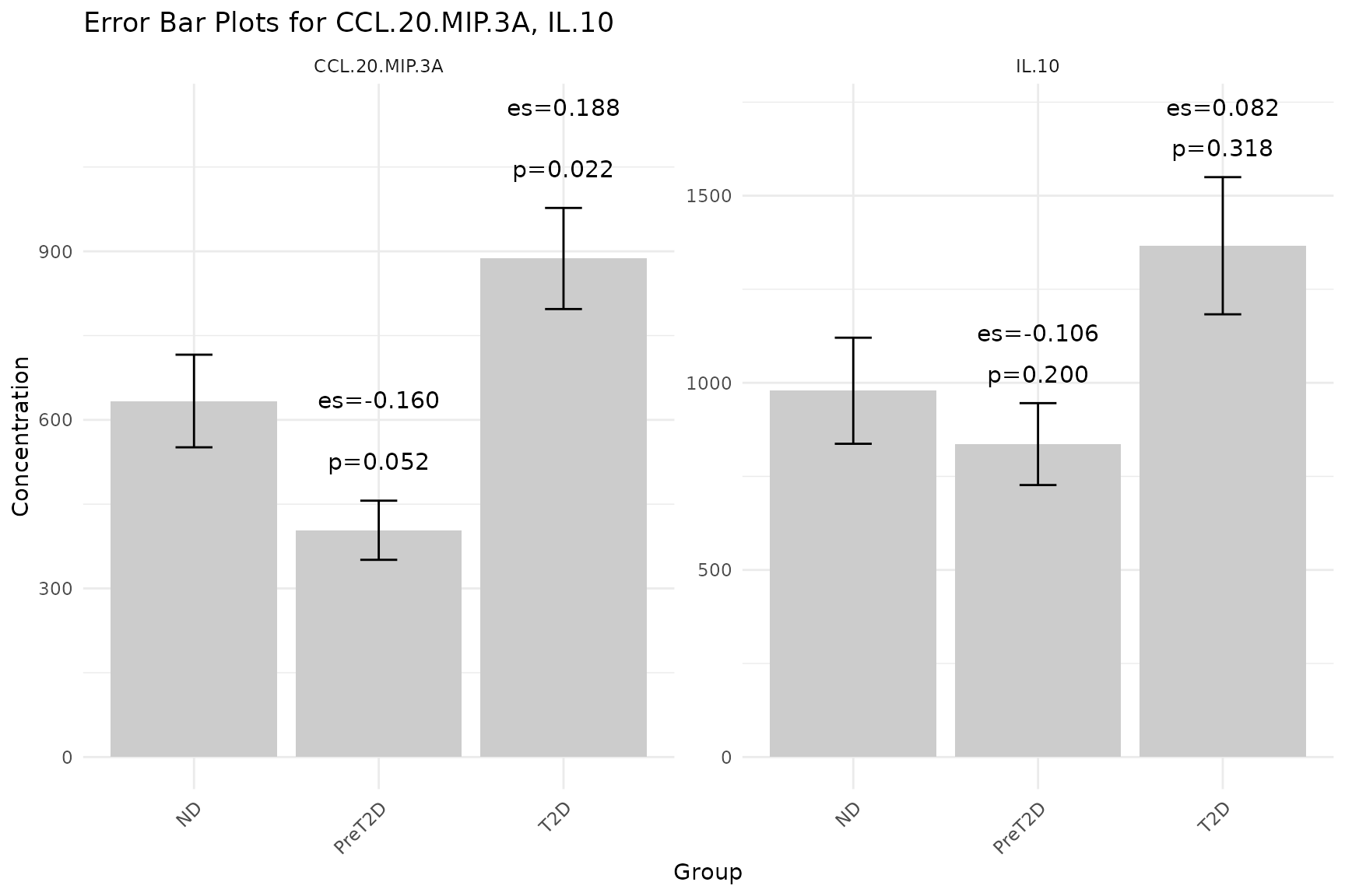
2.4 Error Bar Plots - cyt_errbp()
Purpose: Visualize the central tendency and spread of each cytokine across groups, with optional statistical annotations (p-values and effect sizes) comparing each group to the first (baseline) group.
Key data requirements: - At least one numeric column
and one grouping column. - The first factor level of
group_col is used as the baseline for comparisons.
Key parameters:
| Parameter | Description | Default |
|---|---|---|
group_col |
Name of the grouping column | - |
stat |
Central tendency: "mean" or "median"
|
"mean" |
error |
Spread: "se" (standard error), "sd",
"mad", "ci" (95% CI) |
"se" |
scale |
Data transformation (see cyt_bp()) |
"none" |
method |
Statistical test: "auto", "ttest",
"wilcox"
|
"auto" |
p_lab |
Show p-value annotations | TRUE |
es_lab |
Show effect size annotations | TRUE |
class_symbol |
Use symbols (*, >>) rather than
numeric values |
FALSE |
p_adjust_method |
p-value correction method (e.g. "BH") |
NULL |
output_file |
File path to save | NULL |
Interpreting the output: - Each facet panel
corresponds to one cytokine. Bars show the central tendency; error bars
show spread. - P-value labels above bars indicate statistical
significance versus the baseline group. Values
0.05 are conventionally significant. - Effect size labels indicate the
practical magnitude of the difference: larger absolute values denote
greater differences. For t-test comparisons, this is Cohen’s d; for
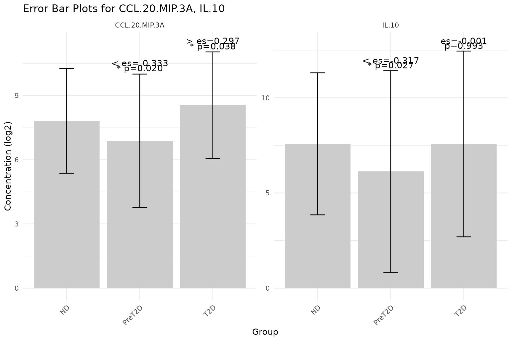
Wilcoxon, the rank-biserial correlation. -
class_symbol = TRUE renders significance as stars
(* to *****) and effect size as arrows
(> to >>>>>), following
conventions used in the accompanying publication.
# Basic error bar plot: default mean +/- SE
df_err <- ExampleData1[, c("Group", "CCL-20/MIP-3A", "IL-10")]
cyt_errbp(
  df_err,
  group_col = "Group",
  x_lab = "Group",
  y_lab = "Concentration"
)
# Mean +/- SD with log2 transformation, symbols, and t-test
cyt_errbp(
  df_err,
  group_col = "Group",
  stat = "mean",
  error = "sd",
  scale = "log2",
  class_symbol = TRUE,
  method = "ttest",
  x_lab = "Group",
  y_lab = "Concentration (log2)"
)
Tip: Use
p_adjust_method = "BH"when analysing a large cytokine panel to control the false discovery rate across multiple comparisons.
3. Univariate Analysis
3.1 Two-group comparisons - cyt_univariate()
Purpose: Perform pairwise statistical tests between exactly two groups for each numeric cytokine column. For each categorical predictor with exactly two levels, either a Student’s t-test or Wilcoxon rank-sum test is applied to each numeric outcome.
Key data requirements: - At least one factor/character column with exactly two levels. - At least one numeric column. - Both groups must have 2 observations with non-zero variance.
Automatic test selection
(method = "auto"): When
method = "auto", a Shapiro-Wilk normality test is applied
to the pooled values for each cytokine within a comparison. If both
groups pass normality (p > 0.05), a t-test is used; otherwise, the
Wilcoxon rank-sum (Mann-Whitney U) test is used. This selection is done
independently for each cytokine. If you prefer a consistent approach,
set method = "ttest" or method = "wilcox"
explicitly.
Key parameters:
| Parameter | Description | Default |
|---|---|---|
scale |
Transformation applied before testing | NULL |
method |
"auto", "ttest", or
"wilcox"
|
"auto" |
format_output |
Return as tidy data frame (TRUE) or list of test
objects (FALSE) |
FALSE |
p_adjust_method |
Multiple testing correction (e.g. "BH") |
NULL |
Interpreting the output: - With
format_output = TRUE, a data frame is returned with
columns: Outcome (cytokine), Categorical
(grouping variable), Comparison (group A vs group B),
Test (method used), Estimate,
Statistic, and P_value. - P-values < 0.05
indicate a statistically significant difference between groups for that
cytokine. - When testing many cytokines simultaneously, use
p_adjust_method = "BH" to control the false discovery rate;
the adjusted column P_adj will be appended.
data_uni <- ExampleData1[, -c(3)]
data_uni <- dplyr::filter(data_uni, Group != "ND", Treatment != "Unstimulated")

# Tidy output with log2 transformation and automatic test selection
cyt_univariate(
  data_uni[, c("Group", "Treatment", "IL-10", "CCL-20/MIP-3A")],
  scale    = "log2",
  method   = "auto",
  format_output = TRUE,
  p_adjust_method = "BH"
)
#>         Outcome Categorical      Comparison
#> 1         IL.10       Group   PreT2D vs T2D
#> 2 CCL.20.MIP.3A       Group   PreT2D vs T2D
#> 3         IL.10   Treatment CD3/CD28 vs LPS
#> 4 CCL.20.MIP.3A   Treatment CD3/CD28 vs LPS
#>                                                Test Estimate Statistic P_value
#> 1 Wilcoxon rank sum test with continuity correction   -0.956    1625.0   0.012
#> 2 Wilcoxon rank sum test with continuity correction   -1.575    1050.5   0.000
#> 3 Wilcoxon rank sum test with continuity correction    1.690    3091.0   0.000
#> 4 Wilcoxon rank sum test with continuity correction    0.488    2509.5   0.132
#>   P_adj
#> 1 0.016
#> 2 0.000
#> 3 0.000
#> 4 0.132
3.2 Multi-group comparisons -
cyt_univariate_multi()
Purpose: Extend univariate testing to categorical predictors with more than two levels using either ANOVA (parametric) or Kruskal-Wallis (non-parametric) global tests, followed by pairwise post-hoc comparisons.
Key data requirements: - At least one factor/character column with more than two levels. - At least one numeric column. - ANOVA is restricted to predictors with 10 levels.
Key parameters:
| Parameter | Description | Default |
|---|---|---|
method |
"anova" (Tukey HSD post-hoc) or "kruskal"
(pairwise Wilcoxon) |
"anova" |
cat_vars |
Character vector of categorical column names to test |
NULL (auto-detect) |
cont_vars |
Character vector of numeric column names to test |
NULL (auto-detect) |
p_adjust_method |
Correction method for pairwise p-values | "BH" |
format_output |
Return as tidy data frame | FALSE |
Interpreting the output: - With
format_output = TRUE, a data frame with columns
Outcome, Categorical, Comparison,
and P_adj is returned. - Each row represents one pairwise
comparison for one cytokine. P_adj values < 0.05
indicate significant pairwise differences after multiple testing
correction. - Use method = "kruskal" when cytokine data are
non-normal or when sample sizes are small.
# Kruskal-Wallis with pairwise Wilcoxon for multi-group comparison
cyt_univariate_multi(
  ExampleData1[, c("Group", "IL-10", "CCL-20/MIP-3A")],
  method = "kruskal",
  format_output = TRUE
)
#>         Outcome Categorical Comparison  P_adj
#> 1         IL.10       Group  PreT2D-ND 0.2995
#> 2         IL.10       Group     T2D-ND 0.3181
#> 3         IL.10       Group T2D-PreT2D 0.0849
#> 4 CCL.20.MIP.3A       Group  PreT2D-ND 0.0518
#> 5 CCL.20.MIP.3A       Group     T2D-ND 0.0332
#> 6 CCL.20.MIP.3A       Group T2D-PreT2D 0.0001
4. Statistical Visualizations
4.1 Volcano Plot - cyt_volc()
Purpose: Visualize fold change versus statistical significance for all cytokines between two groups simultaneously, highlighting cytokines that are both biologically meaningful (large fold change) and statistically significant.
Key data requirements: - One grouping column and
multiple numeric columns. - Both conditions specified must exist as
levels of group_col.
Key parameters:
| Parameter | Description | Default |
|---|---|---|
group_col |
Grouping column name | - |
cond1, cond2
|
The two conditions to compare |
NULL (all pairwise) |
fold_change_thresh |
Fold change threshold (original scale) | 2 |
p_value_thresh |
p-value significance threshold | 0.05 |
top_labels |
Number of top cytokines to label | 10 |
method |
"ttest" or "wilcox"
|
"ttest" |
p_adjust_method |
Multiple testing correction | NULL |
add_effect |
Compute and return effect sizes | FALSE |
Interpreting the output: - x-axis:
log2 fold change (cond2 / cond1). Positive values indicate higher
expression in cond2; negative values in cond1.
- y-axis: -log10(p-value). Higher values = more
significant. - Dashed lines: Vertical lines mark the
+/-log2 fold change threshold; the horizontal line marks the -log10
p-value threshold. - Red points: Cytokines exceeding
both thresholds - these are the candidates most likely to be
biologically relevant between the two conditions. -
Labels: The top_labels cytokines with the
most significant p-values are labelled.
data_volc <- ExampleData1[, -c(2:3)]

volc_plots <- cyt_volc(
  data_volc,
  group_col = "Group",
  cond1 = "T2D",
  cond2 = "ND",
  fold_change_thresh = 2.0,
  p_value_thresh = 0.05,
  top_labels = 15,
  method = "ttest"
)

# The function returns a named list of ggplot objects; print the comparison
volc_plots[["T2D vs ND"]]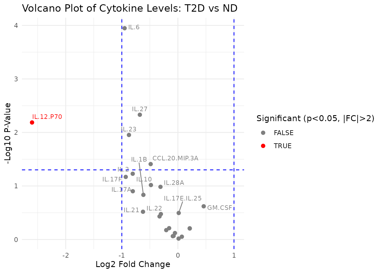
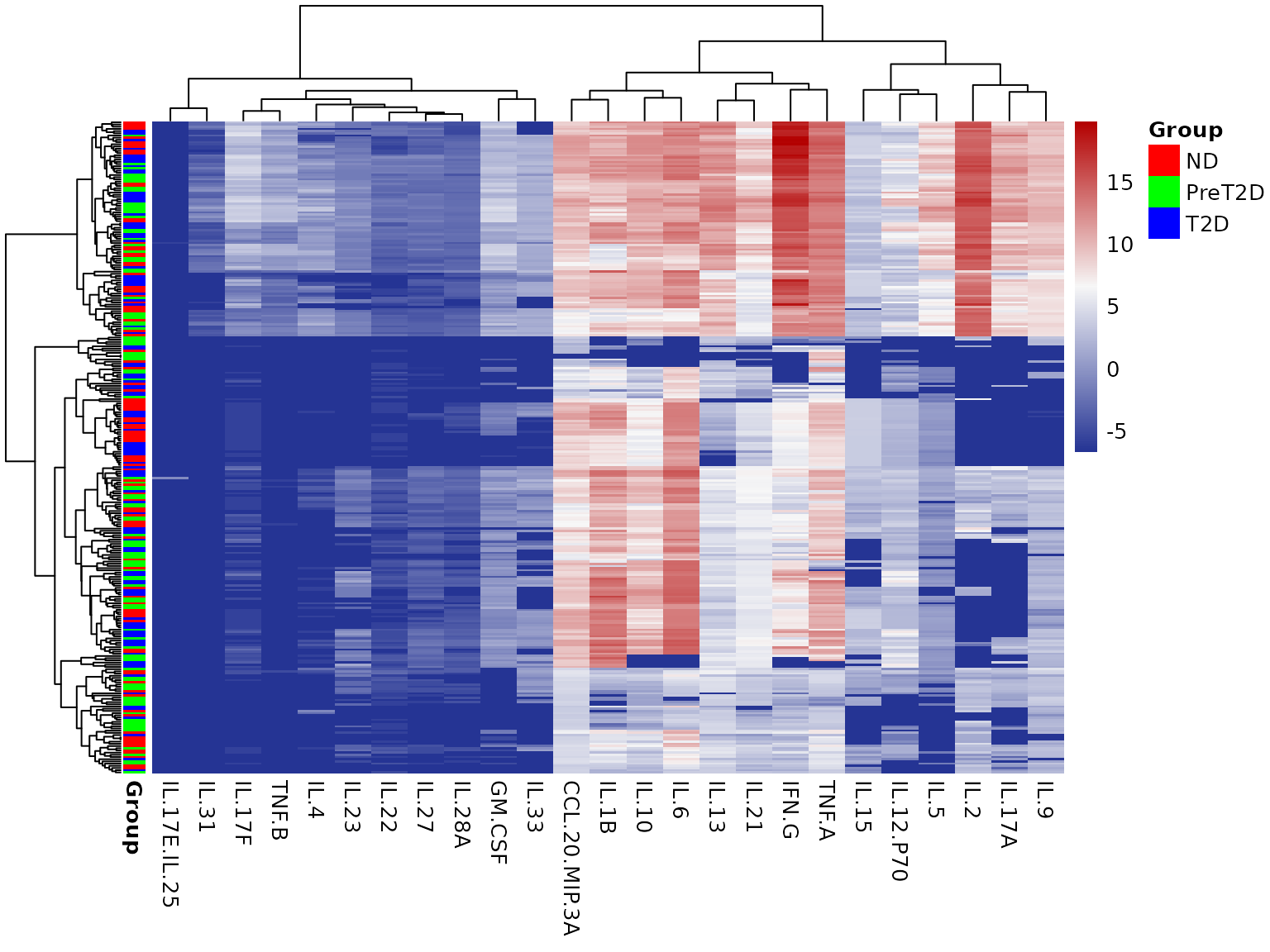
4.2 Heatmap - cyt_heatmap()
Purpose: Visualize the expression matrix of all cytokines across all samples, with optional annotation and hierarchical clustering to reveal sample groupings and cytokine co-expression patterns.
Key data requirements: - A data frame containing numeric cytokine columns. Non-numeric columns are ignored. - The annotation column (if used) must have length equal to the number of rows in the numeric matrix.
Key parameters:
| Parameter | Description | Default |
|---|---|---|
scale |
Transformation: "log2", "log10",
"row_zscore", "col_zscore",
"zscore"
|
NULL |
annotation_col |
Column name or vector for row/column annotation | NULL |
annotation_side |
"auto", "row", or "col"
|
"auto" |
show_row_names |
Show sample row labels | FALSE |
show_col_names |
Show cytokine column labels | TRUE |
cluster_rows |
Cluster samples (rows) | TRUE |
cluster_cols |
Cluster cytokines (columns) | TRUE |
title |
Plot title, or a file path ending in
.pdf/.png to save |
NULL |
Interpreting the output: - The color scale
represents cytokine expression after any transformation: blue = low,
white = mid, red = high. - Row dendrogram (left) clusters samples by
their cytokine expression profiles. Samples that cluster together share
similar cytokine signatures. - Column dendrogram (top) clusters
cytokines by co-expression. Cytokines close together in the column
dendrogram are correlated across samples. - The annotation sidebar (if
provided) color-codes samples by group, making it easy to see whether
cluster structure aligns with biological groupings. - Hiding row names
(show_row_names = FALSE) is recommended when there are many
samples, as individual sample labels become unreadable and clutter the
plot.
cyt_heatmap(
  data = data_df[, -c(2:3)],
  scale = "log2",
  annotation_col = "Group",
  annotation_side = "auto",
  show_row_names = FALSE,
  title = NULL
)
4.3 Dual-Flashlight Plot - cyt_dualflashplot()
Purpose: Simultaneously visualize effect size (SSMD - Strictly Standardized Mean Difference) and fold change for all cytokines between two groups. The dual-flashlight plot is particularly valuable for identifying cytokines with both a large effect size and substantial fold change, which are strong candidates for further investigation as biomarkers.
Why SSMD instead of p-values? Traditional p-values conflate effect size with sample size: a very large study can yield significant p-values for biologically trivial differences. SSMD quantifies effect size independently of sample size, making it suitable for prioritizing cytokines in panels of varying sizes.
Key data requirements: - A data frame with numeric
cytokine columns and one grouping column. - group1 and
group2 must be levels present in
group_var.
Key parameters:
| Parameter | Description | Default |
|---|---|---|
group_var |
Grouping column name | - |
group1, group2
|
The two conditions to compare | - |
ssmd_thresh |
SSMD threshold for marking significance | 1 |
log2fc_thresh |
log2 fold change threshold | 1 |
top_labels |
Number of cytokines with largest | SSMD |
verbose |
Print the underlying statistics table | FALSE |
Interpreting the output: - x-axis:
Average log2 fold change. Positive = higher in group1. -
y-axis: SSMD. |SSMD|
1 = strong effect; |SSMD|
0.5 = moderate. - Point color: Effect strength category
(strong = red, moderate = orange, weak = blue). - Point
shape: Triangles indicate cytokines that exceed both the SSMD
and log2FC thresholds simultaneously - these are the most compelling
candidates. - Dashed lines: Mark the defined
thresholds. - Cytokines in the upper-right and lower-left quadrants
beyond the dashed lines are elevated in group1 or
group2 respectively, with strong effect and substantial
fold change.
data_dfp <- ExampleData1[, -c(2:3)]

dfp <- cyt_dualflashplot(
  data_dfp,
  group_var    = "Group",
  group1       = "T2D",
  group2       = "ND",
  ssmd_thresh  = 0.2,
  log2fc_thresh = 1,
  top_labels   = 10,
  verbose      = FALSE
)
dfp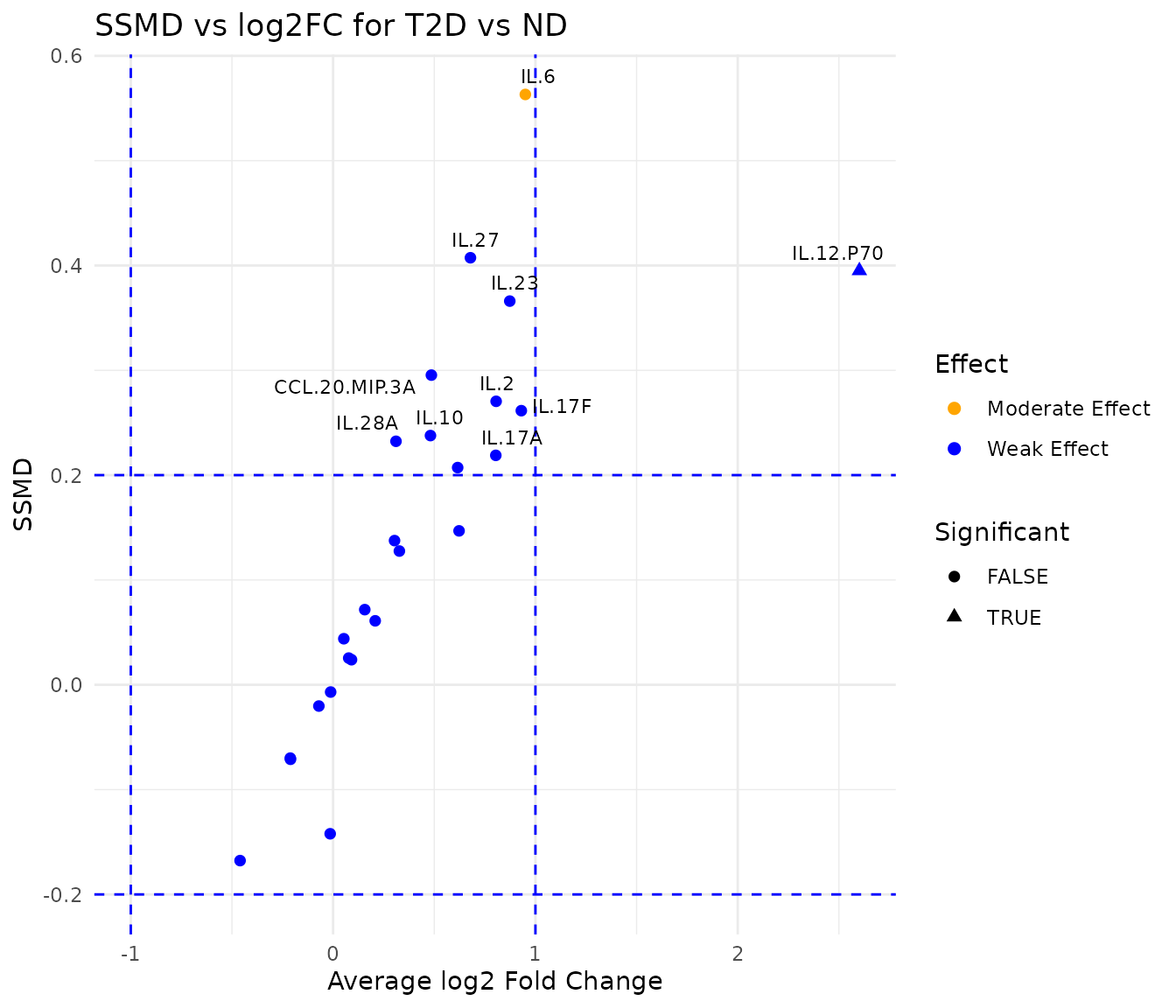
# Inspect the underlying statistics
head(dfp$data[order(abs(dfp$data$ssmd), decreasing = TRUE), ], 10)
#> # A tibble: 10 × 11
#>    cytokine        mean_ND mean_PreT2D   mean_T2D variance_ND variance_PreT2D
#>    <chr>             <dbl>       <dbl>      <dbl>       <dbl>           <dbl>
#>  1 IL.6          4620.       5197.      8925.         2.86e+7         5.72e+7
#>  2 IL.27            0.0662      0.0834     0.106      6.18e-3         5.66e-3
#>  3 IL.12.P70       13.0        39.1       78.9        4.15e+2         2.56e+4
#>  4 IL.23            0.147       0.243      0.269      3.13e-2         9.37e-2
#>  5 CCL.20.MIP.3A  634.        404.       887.         6.72e+5         2.74e+5
#>  6 IL.2          9227.      10718.     16129.         2.60e+8         4.10e+8
#>  7 IL.17F           1.63        2.35       3.11       1.56e+1         3.37e+1
#>  8 IL.10          979.        836.      1366.         1.99e+6         1.19e+6
#>  9 IL.28A           0.0537      0.0710     0.0666     2.45e-3         5.10e-3
#> 10 IL.17A         352.        653.       615.         9.40e+5         2.88e+6
#> # ℹ 5 more variables: variance_T2D <dbl>, ssmd <dbl>, log2FC <dbl>,
#> #   Effect <fct>, Significant <lgl>
5. Multivariate Analysis
5.1 Principal Component Analysis - cyt_pca()
Purpose: Reduce the dimensionality of the cytokine data and visualize sample-level variation across groups. PCA identifies the axes (principal components) of greatest variance in the data without using group labels, making it an unsupervised method suitable for initial exploration.
Key data requirements: - At least one grouping column and multiple numeric cytokine columns. - A sufficient number of observations relative to the number of cytokines is recommended (at least n > p, ideally n > 3p).
Key parameters:
| Parameter | Description | Default |
|---|---|---|
group_col |
Primary grouping column | - |
group_col2 |
Second grouping column (stratifies analysis) | NULL |
colors |
Vector of colors for groups |
NULL (auto) |
pch_values |
Vector of point shapes, one per group level | required |
comp_num |
Number of principal components to compute | 2 |
ellipse |
Draw 95% confidence ellipses per group | FALSE |
scale |
Data transformation | "none" |
style |
Set to "3D" for a 3D scatter if
comp_num = 3
|
NULL |
output_file |
File path to save all plots | - |
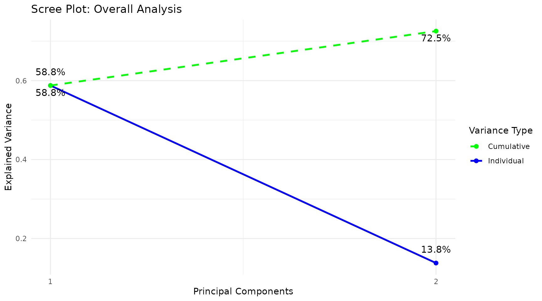
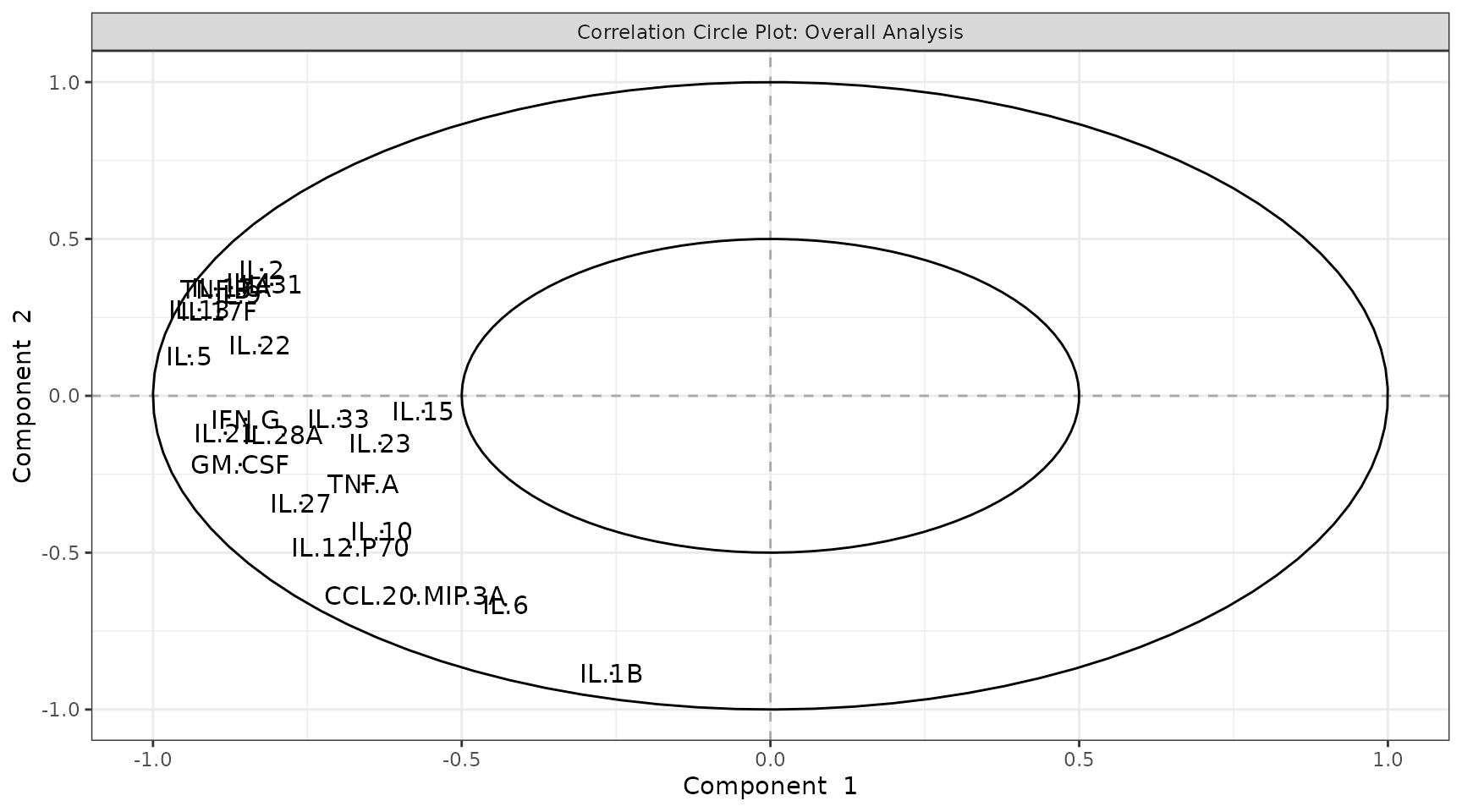
Interpreting the output: - Individuals plot: Each point is one sample. Points close together have similar cytokine profiles. Clear separation between colored groups suggests a discriminating cytokine signature exists. - Scree plot: Shows the percentage of variance explained by each component (individual, blue) and cumulatively (dashed green). Choose the number of components that capture 70-80% of variance. - Loadings plot: Shows which cytokines contribute most to each component. Long bars = large contribution. The sign indicates direction (positive loading = higher values push samples in the positive direction along that component). - Biplot: Overlays sample scores and cytokine loadings. Cytokine arrows pointing toward a group cluster indicate those cytokines are elevated in that group. - Correlation circle: Cytokines near the edge of the circle are well represented by the selected two components. Cytokines close together are positively correlated; those opposite are negatively correlated.
data_pca <- ExampleData1[, -c(3, 23)]
data_pca <- dplyr::filter(data_pca, Group != "ND" & Treatment != "Unstimulated")

pca_results <- cyt_pca(
  data_pca,
  output_file  = NULL,
  colors       = c("black", "red2"),
  scale        = "log2",
  comp_num     = 2,
  pch_values   = c(16, 4),
  group_col    = "Group",
  ellipse      = TRUE
)
pca_results$overall_indiv_plot
pca_results$scree_plot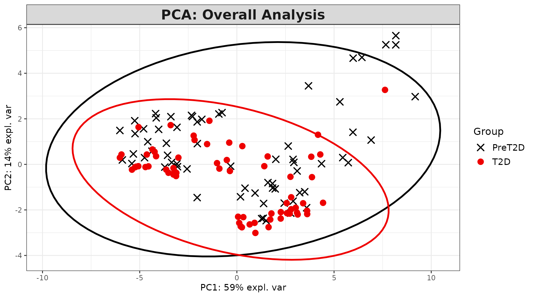
pca_results$loadings$Comp1()
pca_results$correlation_circle()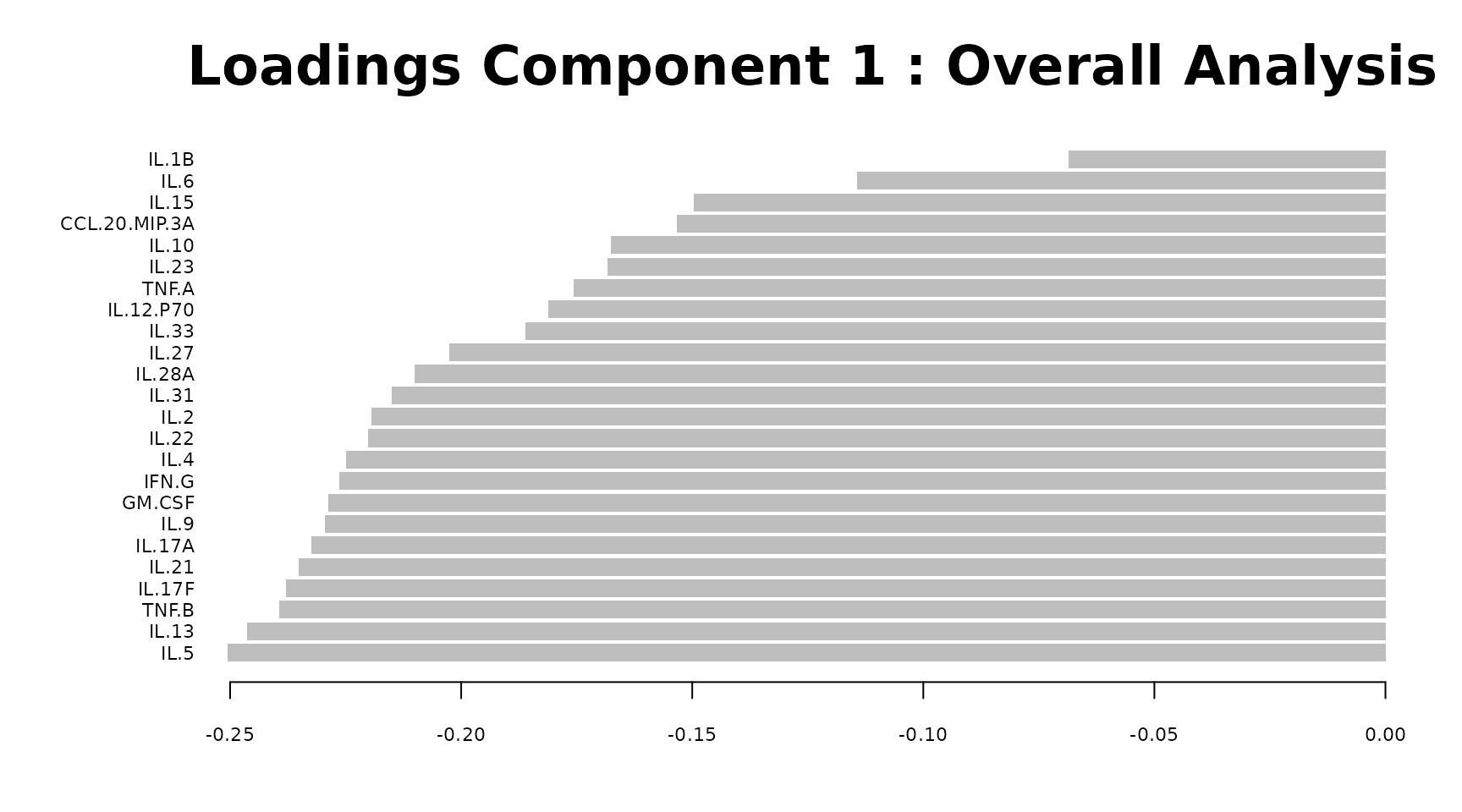
5.2 Sparse PLS-DA - cyt_splsda()
Purpose: A supervised multivariate method that finds linear combinations of cytokines that maximally discriminate between groups, while simultaneously selecting the most discriminating cytokines (sparsity). Unlike PCA, sPLS-DA uses group labels to guide the component construction.
Key data requirements: - At least two groups in
group_col. - Multiple numeric cytokine columns. - For
reliable cross-validation,
10 samples per group is recommended.
Key parameters:
| Parameter | Description | Default |
|---|---|---|
group_col |
Primary grouping column | - |
group_col2 |
Treatment/stratification column (runs analysis per level) | NULL |
var_num |
Number of cytokines selected per component | required |
comp_num |
Number of components | 2 |
pch_values |
Point shapes, one per group | required |
cv_opt |
Cross-validation: "loocv" or "Mfold"
|
NULL |
fold_num |
Number of folds for Mfold CV | 5 |
tune |
Auto-tune var_num and comp_num via CV |
FALSE |
ellipse |
Draw 95% confidence ellipses | FALSE |
bg |
Draw prediction background | FALSE |
roc |
Plot ROC curves | FALSE |
scale |
Data transformation | "none" |
Interpreting the output: - Classification
plot (individuals plot): Labelled with accuracy (% training
samples correctly classified). Clear separation indicates the model
successfully identified a discriminating cytokine signature. -
Loadings plot: Shows which cytokines load most strongly
on each component and in which group they are elevated (color of the
bar). The contrib = "max" setting colors each bar by the
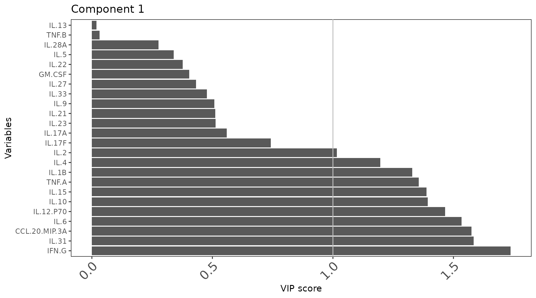
group with the highest mean for that cytokine. - VIP scores
plot: Variable Importance in Projection scores for each
component. Cytokines with VIP > 1 are considered important
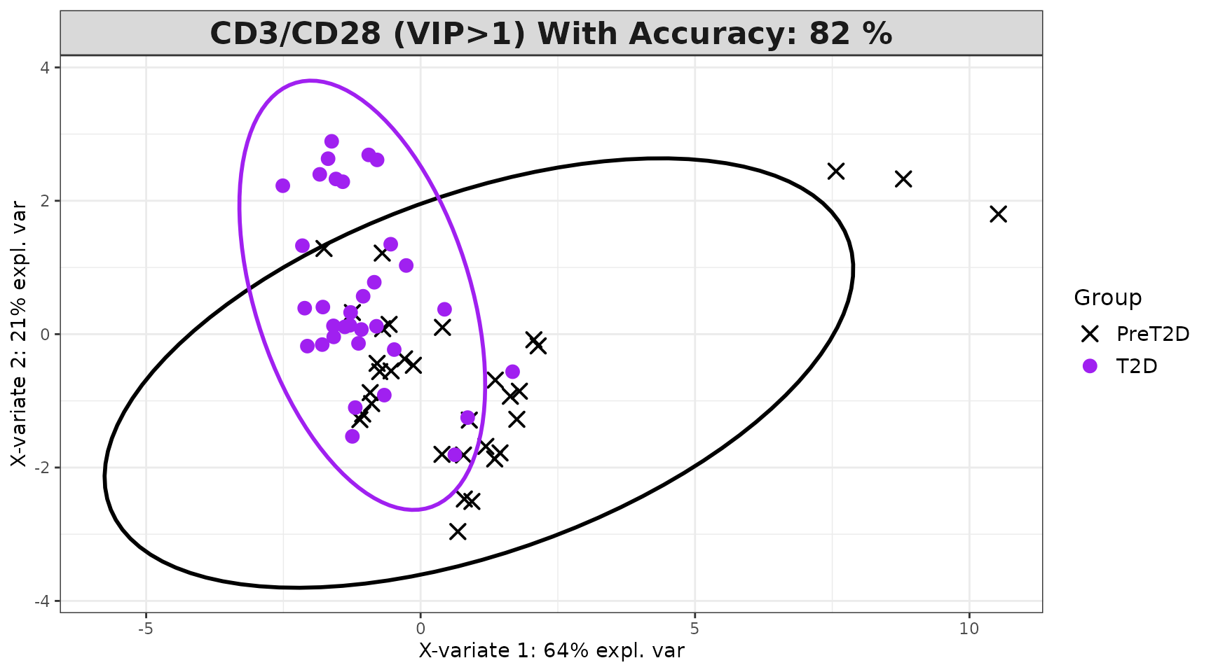
discriminators and are used to fit a refined model. - VIP > 1
classification plot: A second model fitted using only VIP >
1 cytokines. Comparing accuracy between the full and VIP-filtered model
shows whether the signature can be simplified. -
Cross-validation error plot (if cv_opt is
set): Error rate across components. The optimal number of components is
where the error rate plateaus or reaches its minimum.
data_spls <- ExampleData1[, -c(3)]
data_spls <- dplyr::filter(data_spls, Group != "ND" & Treatment == "CD3/CD28")

spls_results <- cyt_splsda(
  data_spls,
  output_file  = NULL,
  colors       = c("black", "purple"),
  scale        = "log2",
  ellipse      = TRUE,
  var_num      = 25,
  cv_opt       = "loocv",
  comp_num     = 2,
  pch_values   = c(16, 4),
  group_col    = "Group",
  group_col2   = "Treatment",
  roc          = FALSE,
  verbose      = FALSE
)
spls_results$overall_indiv_plot
spls_results$vip_indiv_plot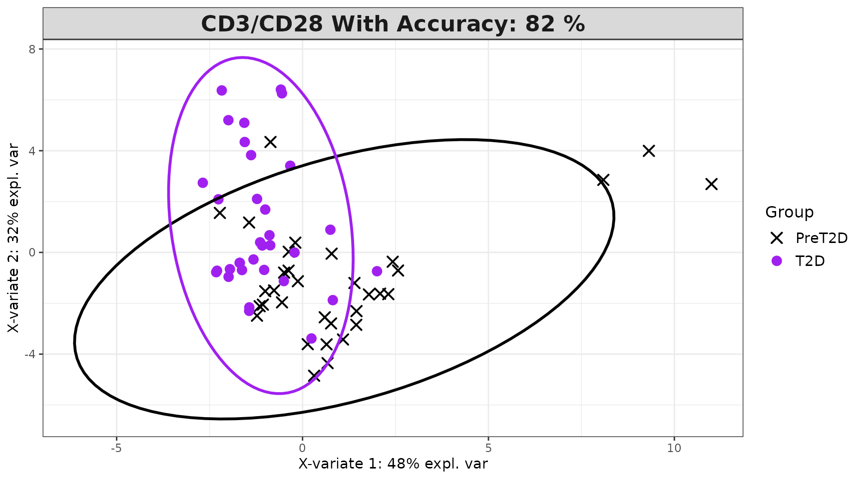
spls_results$loadings$Comp1()
spls_results$vip_scores$Comp1()
5.3 MINT sPLS-DA - cyt_mint_splsda()
Purpose: An extension of sPLS-DA for datasets collected across multiple batches or studies. MINT (Multivariate INTegration) models a global biological signal while accounting for batch-specific variation, making it appropriate when data cannot be combined directly due to technical differences between collection sites or time points.
Key data requirements: - Same as
cyt_splsda(), plus a batch_col column
identifying which batch/study each sample belongs to. - At least two
batches are required; each batch should contain samples from all groups
if possible.
Key parameters: Same as cyt_splsda(),
plus:
| Parameter | Description | Default |
|---|---|---|
batch_col |
Column identifying batch/study membership | required |
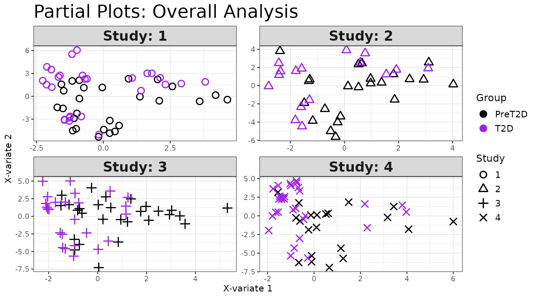
Interpreting the output: - Identical to
cyt_splsda() outputs, with the addition of partial
plots (one per batch), which show how well the global model
fits within each individual batch. - The global individuals plot should
show separation between groups even when batch effects are present - if
groups overlap only in the global plot but separate in partial plots,
the batch effect is dominating the signal.
data_mint <- ExampleData5[, -c(2, 4)]
data_mint <- dplyr::filter(data_mint, Group != "ND")

mint_results <- cyt_mint_splsda(
  data_mint,
  group_col  = "Group",
  batch_col  = "Batch",
  colors     = c("black", "purple"),
  ellipse    = TRUE,
  var_num    = 25,
  comp_num   = 2,
  scale      = "log2",
  verbose    = FALSE
)
mint_results$global_indiv_plot
mint_results$partial_indiv_plot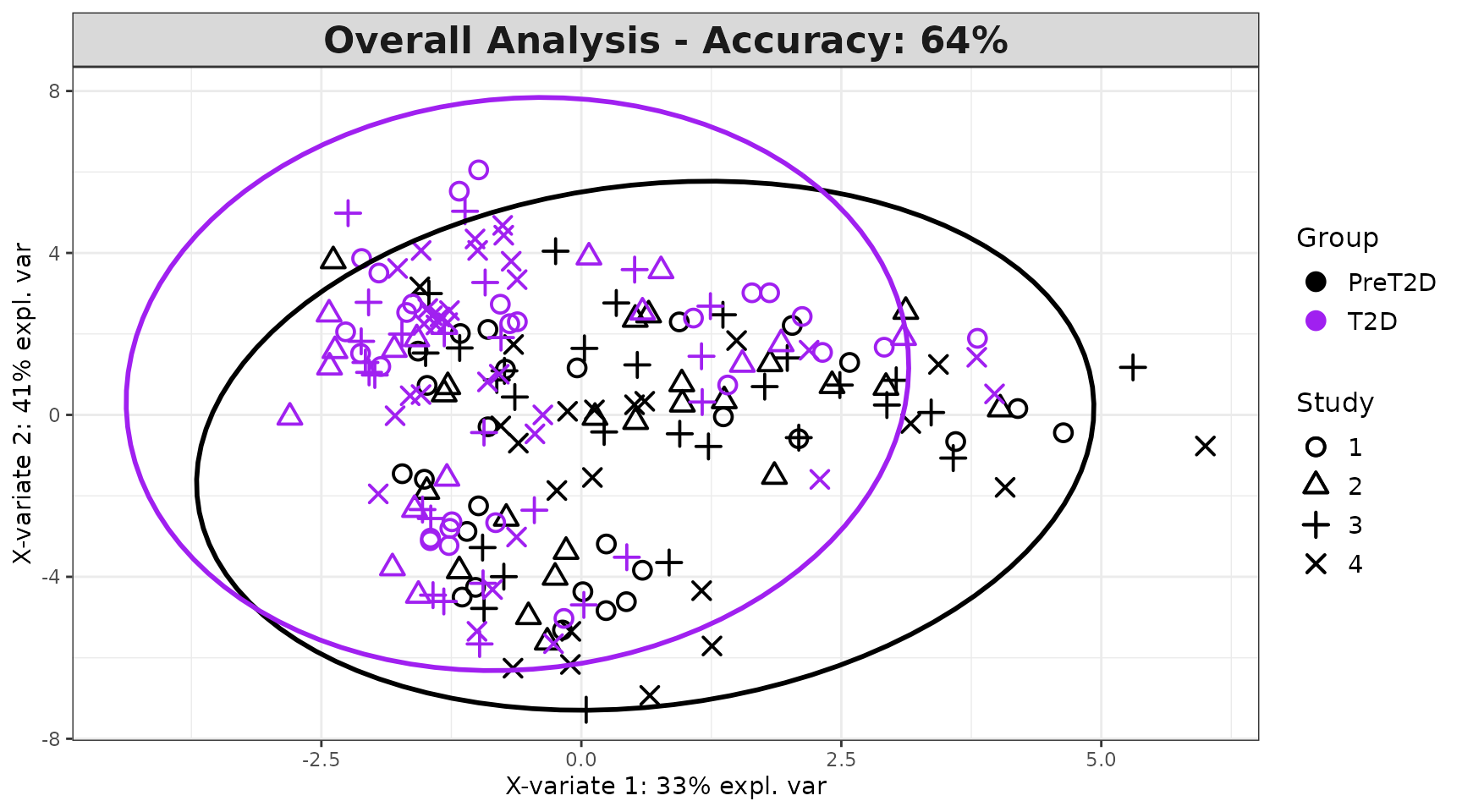
mint_results$global_loadings_plots$Comp1()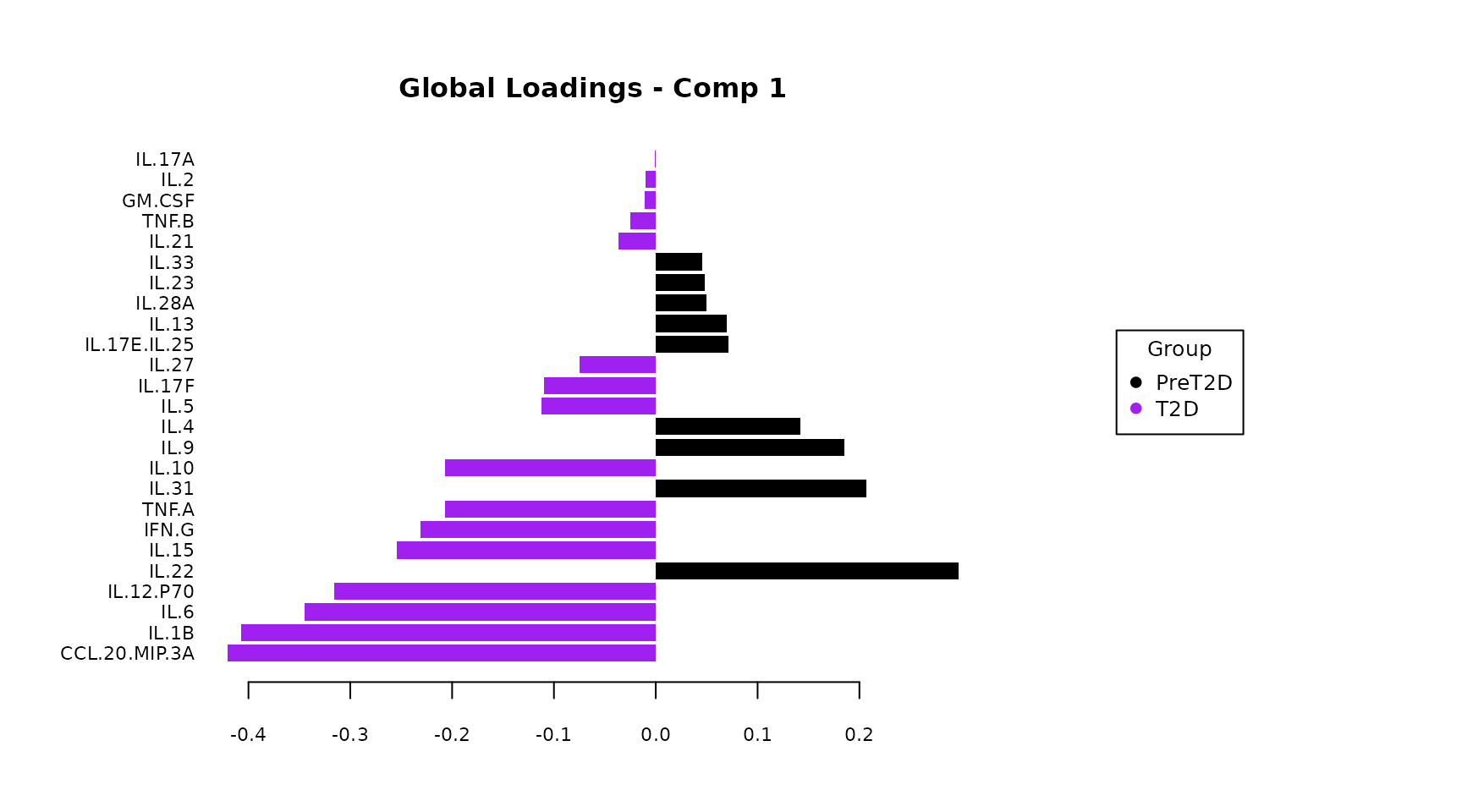
6. Machine Learning Models
Recommended sample size: For reliable performance estimates, machine learning methods require larger datasets. A minimum of 20 samples per class is recommended; cross-validation estimates become stable with 50 samples per class.
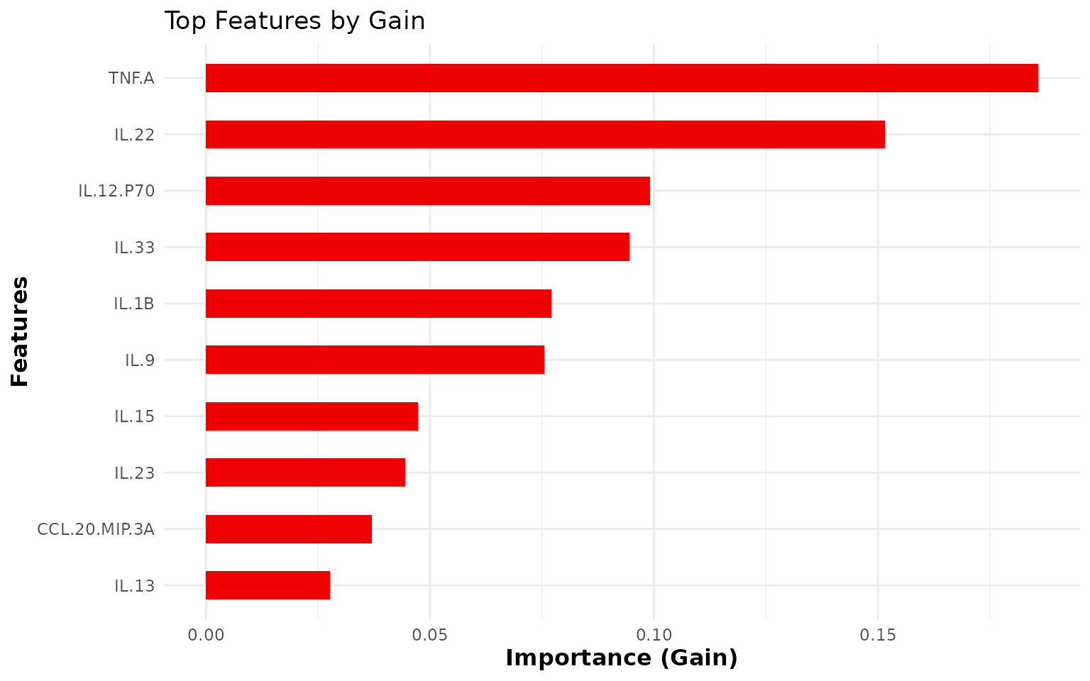
6.1 XGBoost Classification - cyt_xgb()
Purpose: Train a gradient-boosted tree classifier on cytokine data for multi-class or binary group classification. XGBoost is well suited to high-dimensional cytokine panels and provides feature importance as a by-product.
Key data requirements: - One grouping column (the outcome) and multiple numeric cytokine predictors. - Grouping column will be encoded to numeric labels internally (0-indexed).
Key parameters:
| Parameter | Description | Default |
|---|---|---|
group_col |
Outcome column name | - |
train_fraction |
Proportion used for training | 0.7 |
nrounds |
Number of boosting rounds | 500 |
max_depth |
Maximum tree depth | 6 |
learning_rate |
Step size shrinkage | 0.1 |
cv |
Run k-fold cross-validation | FALSE |
nfold |
Number of CV folds | 5 |
objective |
Loss function: "multi:softprob" or
"binary:logistic"
|
"multi:softprob" |
eval_metric |
Evaluation metric during training | "mlogloss" |
plot_roc |
Plot ROC curve (binary only) | FALSE |
top_n_features |
Number of features shown in importance plot | 10 |
scale |
Data transformation | "none" |
Note on Ckmeans.1d.dp: The
xgb.ggplot.importance() function optionally uses the
Ckmeans.1d.dp package for a clustered importance plot. If
this package is not installed, cyt_xgb() will automatically
fall back to a standard bar chart. Install it with
install.packages("Ckmeans.1d.dp") for the enhanced
plot.
Interpreting the output: - Confusion
matrix: Rows = actual classes; columns = predicted classes. The
diagonal shows correct classifications. Off-diagonal values are
misclassifications. - Feature importance plot: Shows
the top top_n_features cytokines ranked by Gain (the
improvement in the loss function attributable to each feature).
Cytokines with higher Gain are more important for classification. -
Cross-validation accuracy (if cv = TRUE):
Provides an estimate of out-of-sample performance less susceptible to
overfitting than training accuracy alone. - ROC curve
(binary only): Area Under the Curve (AUC) summarizes classifier
performance across all thresholds. AUC = 1 is perfect; AUC = 0.5 is no
better than chance.
data_ml <- data.frame(ExampleData1[, 1:3], log2(ExampleData1[, -c(1:3)]))
data_ml <- data_ml[, -c(2:3)]
data_ml <- dplyr::filter(data_ml, Group != "ND")

cyt_xgb(
  data          = data_ml,
  group_col     = "Group",
  nrounds       = 250,
  max_depth     = 4,
  learning_rate = 0.05,
  nfold         = 5,
  cv            = FALSE,
  objective     = "multi:softprob",
  eval_metric   = "mlogloss",
  top_n_features = 10,
  verbose       = 0,
  plot_roc      = FALSE,
  print_results = FALSE,
  seed          = 123
)
6.2 Random Forest Classification - cyt_rf()
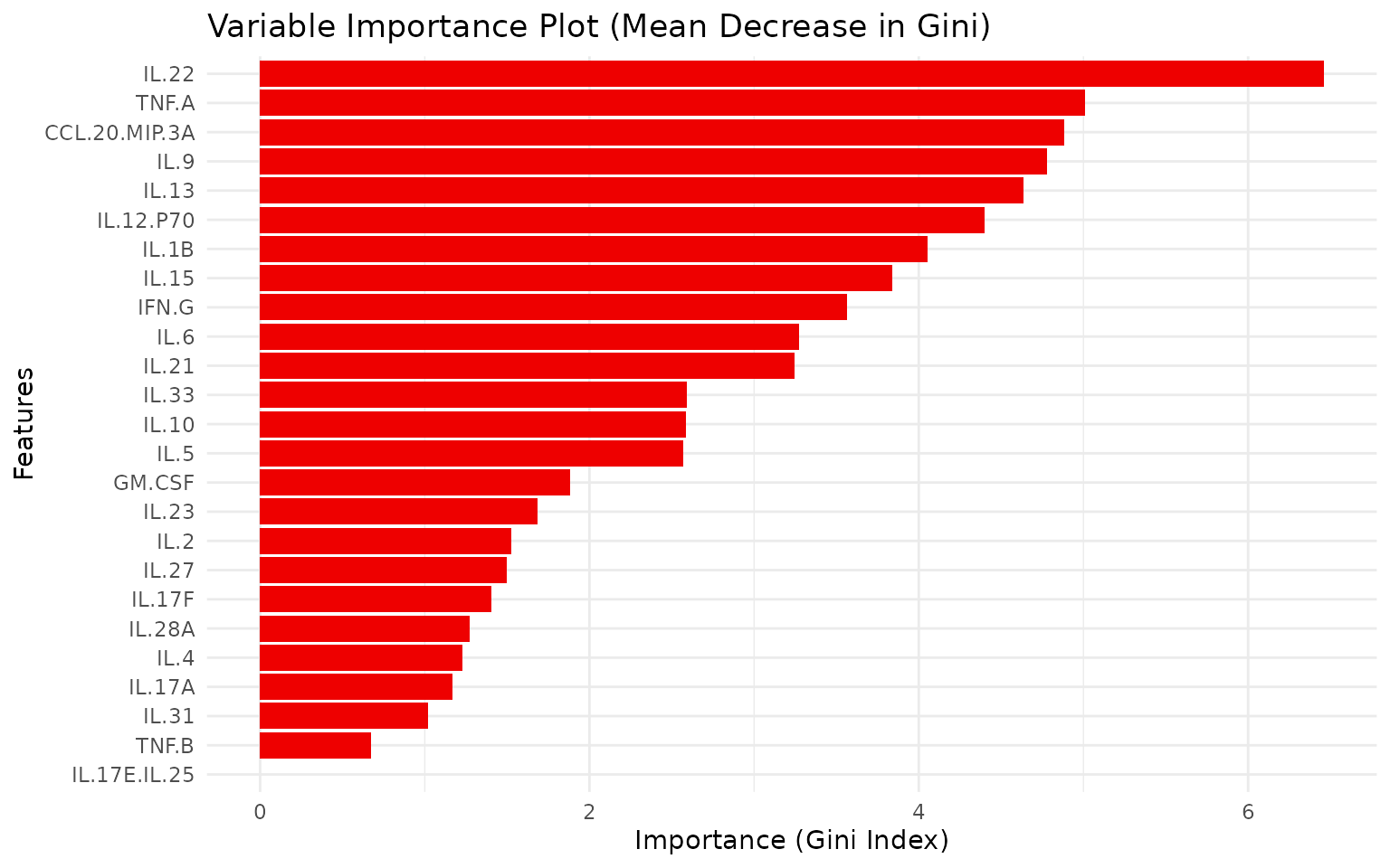
Purpose: Train a random forest ensemble classifier on cytokine data. Random forests are robust to outliers and correlated predictors, and naturally provide variable importance through the mean decrease in Gini impurity.
Key parameters:
| Parameter | Description | Default |
|---|---|---|
group_col |
Outcome column name | - |
ntree |
Number of trees | 500 |
mtry |
Variables tried at each split | 5 |
train_fraction |
Training proportion | 0.7 |
run_rfcv |
Run cross-validation for feature selection | TRUE |
k_folds |
Folds for rfcv
|
5 |
plot_roc |
Plot ROC curve (binary only) | FALSE |
cv |
Run caret k-fold CV | FALSE |
scale |
Data transformation | "none" |
verbose |
Print performance metrics | FALSE |
Interpreting the output: - Variable
importance plot: Cytokines ordered by Mean Decrease in Gini.
Higher values indicate greater discrimination ability. This complements
sPLS-DA loadings as a non-linear importance measure. -
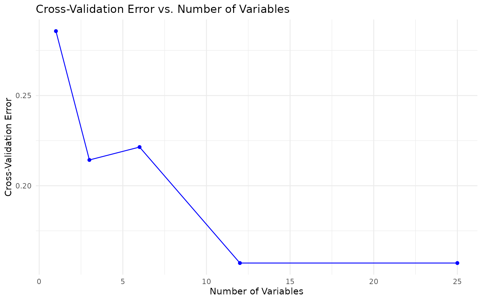
Cross-validation error curve (if
run_rfcv = TRUE): Error rate versus number of variables.
The elbow of this curve (where error stabilizes) suggests the minimum
number of cytokines needed for good classification. This is useful for
building parsimonious panels. - ROC curve (binary
only): Same interpretation as in cyt_xgb().
cyt_rf(
  data       = data_ml,
  group_col  = "Group",
  ntree      = 500,
  mtry       = 4,
  k_folds    = 5,
  run_rfcv   = TRUE,
  plot_roc   = FALSE,
  verbose    = FALSE,
  seed       = 123
)
7. Saving Plots and Exporting Results
Saving plots from individual functions
All plotting functions accept an output_file argument.
The file extension determines the format:
# Save all boxplots to a multi-page PDF
cyt_bp(data_df[, -c(1:3)], output_file = "boxplots.pdf", scale = "log2")

# Save grouped violin plots to PNG
cyt_violin(data_df[, -c(3, 5:28)], group_by = "Group",
           output_file = "violins.png")
Supported formats: .pdf, .png,
.tiff, .svg.
Saving plots from multivariate functions using
cyt_export()
Multivariate functions return lists of ggplot objects
and plot-generating closures. Use cyt_export() to save them
in bulk:
# Save all sPLS-DA plots to a PDF
cyt_export(
  plots    = list(
    spls_results$overall_indiv_plot,
    spls_results$loadings$Comp1,
    spls_results$vip_indiv_plot
  ),
  filename = "splsda_results",
  format   = "pdf"
)

# Or pass output_file directly to the function
cyt_splsda(..., output_file = "splsda_results.pdf")
Modifying returned plots
All functions return ggplot objects invisibly, enabling
further customization:
p <- cyt_bp(data_df[, -c(1:3)], scale = "log2")
# Add a custom title to the first page
p[["page1"]] + ggplot2::ggtitle("My Custom Title") +
  ggplot2::theme(plot.title = ggplot2::element_text(size = 16))
8. Recommended Analysis Workflow
The following workflow is recommended for a typical cytokine profiling study:
- Load and inspect data - check dimensions, column types, and missingness.
-
Assess distributions (
cyt_skku()) - determine whether log2 transformation is warranted. -
Exploratory visualization (
cyt_bp()orcyt_violin(),cyt_errbp()) - identify obvious group differences and data quality issues. -
Univariate testing (
cyt_univariate(),cyt_univariate_multi()) - with FDR correction for panels > 10 cytokines. -
Multivariate exploration (
cyt_pca()) - visualize global structure and assess whether groups separate. -
Supervised discrimination
(
cyt_splsda()) - identify the minimal cytokine signature that discriminates groups; validate with cross-validation. -
Visualization of key findings
(
cyt_volc(),cyt_dualflashplot(),cyt_heatmap()) - summarize significant and high-effect cytokines for reporting. -
Machine learning validation (
cyt_rf(),cyt_xgb()) - obtain independent importance rankings and classification performance estimates.
Session Information
sessionInfo()
#> R version 4.5.2 (2025-10-31)
#> Platform: x86_64-pc-linux-gnu
#> Running under: Ubuntu 24.04.3 LTS
#>
#> Matrix products: default
#> BLAS:   /usr/lib/x86_64-linux-gnu/openblas-pthread/libblas.so.3
#> LAPACK: /usr/lib/x86_64-linux-gnu/openblas-pthread/libopenblasp-r0.3.26.so;  LAPACK version 3.12.0
#>
#> locale:
#>  [1] LC_CTYPE=C.UTF-8       LC_NUMERIC=C           LC_TIME=C.UTF-8
#>  [4] LC_COLLATE=C.UTF-8     LC_MONETARY=C.UTF-8    LC_MESSAGES=C.UTF-8
#>  [7] LC_PAPER=C.UTF-8       LC_NAME=C              LC_ADDRESS=C
#> [10] LC_TELEPHONE=C         LC_MEASUREMENT=C.UTF-8 LC_IDENTIFICATION=C
#>
#> time zone: UTC
#> tzcode source: system (glibc)
#>
#> attached base packages:
#> [1] stats     graphics  grDevices utils     datasets  methods   base
#>
#> other attached packages:
#> [1] dplyr_1.2.0       CytoProfile_0.2.4
#>
#> loaded via a namespace (and not attached):
#>   [1] Rdpack_2.6.6         pROC_1.19.0.1        gridExtra_2.3
#>   [4] tcltk_4.5.2          rlang_1.1.7          magrittr_2.0.4
#>   [7] otel_0.2.0           matrixStats_1.5.0    e1071_1.7-17
#>  [10] compiler_4.5.2       systemfonts_1.3.1    vctrs_0.7.1
#>  [13] reshape2_1.4.5       stringr_1.6.0        pkgconfig_2.0.3
#>  [16] fastmap_1.2.0        Ckmeans.1d.dp_4.3.5  labeling_0.4.3
#>  [19] utf8_1.2.6           rmarkdown_2.30       prodlim_2025.04.28
#>  [22] ragg_1.5.0           purrr_1.2.1          xfun_0.56
#>  [25] randomForest_4.7-1.2 cachem_1.1.0         jsonlite_2.0.0
#>  [28] recipes_1.3.1        BiocParallel_1.44.0  parallel_4.5.2
#>  [31] R6_2.6.1             bslib_0.10.0         stringi_1.8.7
#>  [34] RColorBrewer_1.1-3   parallelly_1.46.1    rpart_4.1.24
#>  [37] lubridate_1.9.5      jquerylib_0.1.4      xgboost_3.2.0.1
#>  [40] Rcpp_1.1.1           iterators_1.0.14     knitr_1.51
#>  [43] future.apply_1.20.2  Matrix_1.7-4         splines_4.5.2
#>  [46] nnet_7.3-20          igraph_2.2.2         timechange_0.4.0
#>  [49] tidyselect_1.2.1     yaml_2.3.12          timeDate_4052.112
#>  [52] codetools_0.2-20     misc3d_0.9-2         listenv_0.10.0
#>  [55] lattice_0.22-7       tibble_3.3.1         plyr_1.8.9
#>  [58] withr_3.0.2          rARPACK_0.11-0       S7_0.2.1
#>  [61] evaluate_1.0.5       future_1.69.0        desc_1.4.3
#>  [64] survival_3.8-3       proxy_0.4-29         pillar_1.11.1
#>  [67] foreach_1.5.2        stats4_4.5.2         ellipse_0.5.0
#>  [70] generics_0.1.4       ggplot2_4.0.2        scales_1.4.0
#>  [73] globals_0.19.0       class_7.3-23         glue_1.8.0
#>  [76] pheatmap_1.0.13      tools_4.5.2          data.table_1.18.2.1
#>  [79] RSpectra_0.16-2      ModelMetrics_1.2.2.2 gower_1.0.2
#>  [82] fs_1.6.6             grid_4.5.2           tidyr_1.3.2
#>  [85] rbibutils_2.4.1      ipred_0.9-15         nlme_3.1-168
#>  [88] cli_3.6.5            textshaping_1.0.4    mixOmics_6.34.0
#>  [91] plot3D_1.4.2         lava_1.8.2           corpcor_1.6.10
#>  [94] gtable_0.3.6         sass_0.4.10          digest_0.6.39
#>  [97] caret_7.0-1          ggrepel_0.9.7        htmlwidgets_1.6.4
#> [100] farver_2.1.2         htmltools_0.5.9      pkgdown_2.2.0
#> [103] lifecycle_1.0.5      hardhat_1.4.2        MASS_7.3-65